Predicting Boston House Prices
Source:vignettes/Predicting_Boston_House_Prices.Rmd
Predicting_Boston_House_Prices.Rmd
library(dplyr); library(tidyr); library(purrr) # Data wrangling
library(ggplot2); library(stringr) # Plotting
library(tidyfit)   # Auto-ML modeling
The Boston house prices data set (MASS::Boston) presents
a popular test case for regression algorithms. In this article, I assess
the relative performance of 15 different linear regression techniques
using tidyfit::regress.
Let’s begin by loading the data, and splitting it into equally sized training and test sets:
data <- MASS::Boston

# For reproducibility
set.seed(123)
ix_tst <- sample(1:nrow(data), round(nrow(data)*0.5))

data_trn <- data[-ix_tst,]
data_tst <- data[ix_tst,]

as_tibble(data)
#> # A tibble: 506 × 14
#>       crim    zn indus  chas   nox    rm   age   dis   rad   tax ptratio black
#>      <dbl> <dbl> <dbl> <int> <dbl> <dbl> <dbl> <dbl> <int> <dbl>   <dbl> <dbl>
#>  1 0.00632  18    2.31     0 0.538  6.58  65.2  4.09     1   296    15.3  397.
#>  2 0.0273    0    7.07     0 0.469  6.42  78.9  4.97     2   242    17.8  397.
#>  3 0.0273    0    7.07     0 0.469  7.18  61.1  4.97     2   242    17.8  393.
#>  4 0.0324    0    2.18     0 0.458  7.00  45.8  6.06     3   222    18.7  395.
#>  5 0.0690    0    2.18     0 0.458  7.15  54.2  6.06     3   222    18.7  397.
#>  6 0.0298    0    2.18     0 0.458  6.43  58.7  6.06     3   222    18.7  394.
#>  7 0.0883   12.5  7.87     0 0.524  6.01  66.6  5.56     5   311    15.2  396.
#>  8 0.145    12.5  7.87     0 0.524  6.17  96.1  5.95     5   311    15.2  397.
#>  9 0.211    12.5  7.87     0 0.524  5.63 100    6.08     5   311    15.2  387.
#> 10 0.170    12.5  7.87     0 0.524  6.00  85.9  6.59     5   311    15.2  387.
#> # ℹ 496 more rows
#> # ℹ 2 more variables: lstat <dbl>, medv <dbl>
The aim is to predict the median value of owner-occupied homes
('medv' in the data set) using the remaining columns.1 We will
assess performance using
,
which allows intuitive comparisons of in-sample and out-of-sample
fit.
A simple regression
To establish a baseline, we fit an OLS regression model and examine
the test and training set R-squared. The predict function
can be used to obtain predictions, and yardstick is used to
assess performance. The regression is estimated using
tidyfit::regress. tidyfit::m is a generic
model wrapper that is capable of fitting a large number of different
algorithms:
Let’s create a helper function to assess performance. The helper
function wraps predict and prepares in and out-of-sample
performance stats:
assess <- function(model_frame, data_trn, data_tst) {

  oos <- model_frame |>
    predict(data_tst) |>
    group_by(model, .add = TRUE) |>
    yardstick::rsq_trad(truth, prediction) |>
    mutate(type = "Out-of-sample") |>
    arrange(desc(.estimate))

  is <- model_frame |>
    predict(data_trn) |>
    group_by(model, .add = TRUE) |>
    yardstick::rsq_trad(truth, prediction) |>
    mutate(type = "In-sample")

  return(bind_rows(oos, is))

}

plotter <- function(df) {
  df <- df |>
    mutate(lab = round(.estimate, 2)) |>
    mutate(model = str_wrap(model, 12))
  df |>
    mutate(model = factor(model, levels = unique(df$model))) |>
    ggplot(aes(model, .estimate)) +
    geom_point(aes(color = type), size = 2.5, shape = 4) +
    geom_label(aes(label = lab, color = type), size = 2, nudge_x = 0.35) +
    theme_bw() +
    scale_color_manual(values = c("firebrick", "darkblue")) +
    theme(legend.title = element_blank(),
          axis.title.x = element_blank()) +
    coord_cartesian(ylim = c(0.65, 0.95))
}
Now we plot the resulting metrics:
model_frame |>
  assess(data_trn, data_tst) |>
  plotter()
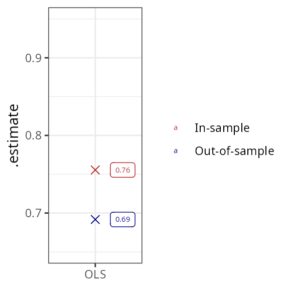
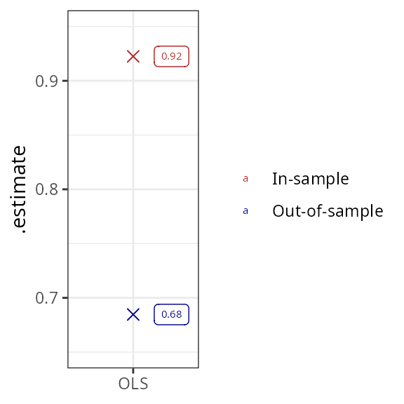
The in-sample fit of the regression is naturally better than out-of-sample, but the difference is not large. The results can be improved substantially by adding interaction terms between features. This leads to a vast improvement in in-sample fit (again, this is a logical consequence of including a large number of regressors), but leads to no improvement in out-of-sample fit, suggesting substantial overfit:
model_frame <- data_trn |>
  regress(medv ~ .*., OLS = m("lm"))

model_frame |>
  assess(data_trn, data_tst) |>
  plotter()
Regularized regression estimators
Regularization controls overfit by introducing parameter bias in exchange for a reduction in estimator variance. A large number of approaches to regularization exist that can be summarized in at least 5 categories:
- Best subset selection
- L1/L2 penalized regression
- Latent factor regression
- Other machine learning
- Bayesian regression
tidyfit includes linear estimators from each of these
categories, as summarized below:
| Best subset | L1/L2 penalized | Latent factors | Machine Learning | Bayesian |
|---|---|---|---|---|
Exhaustive search (leaps)
|
Lasso (glmnet)
|
Principal components regression (pls)
|
Gradient Boosting (mboost)
|
Bayesian regression (arm)
|
Forward selection (leaps)
|
Ridge (glmnet)
|
Partial least squares (pls)
|
Hierarchical feature regression (hfr)
|
Bayesian model averaging (BMS)
|
Backward selection (leaps)
|
ElasticNet (glmnet)
|
Support vector regression (e1071)
|
Bayesian Lasso (monomvn)
|
|
Sequential Replacement (leaps)
|
Adaptive Lasso (glmnet)
|
Bayesian Ridge (monomvn)
|
||
| Genetic Algorithm (‘gaselect’) | Spike and Slab Regression (‘BoomSpikeSlab’) |
In the next code chunk, 17 of the available regression techniques are
fitted to the data set. Hyperparameters are optimized using a 10-fold
cross validation powered by rsample in the background. As a
practical aside, it is possible to set a future plan to
ensure hyperparameter tuning is performed on a parallelized backend.2 This is
done using plan(multisession(workers = n_workers)), where
n_workers is the number of available cores. Furthermore, a
progress bar could be activated using
progressr::handlers(global = TRUE).
model_frame_all <- data_trn |>
  regress(medv ~ .*.,
          OLS = m("lm"),
          BAYES = m("bayes"),
          BMA = m("bma", iter = 10000),
          SEQREP = m("subset", method = "seqrep", IC = "AIC"),
          `FORWARD SELECTION` = m("subset", method = "forward", IC = "AIC"),
          `BACKWARD SELECTION` = m("subset", method = "backward", IC = "AIC"),
          LASSO = m("lasso"),
          BLASSO = m("blasso"),
          SPIKESLAB = m("spikeslab", niter = 10000),
          RIDGE = m("ridge"),
          BRIDGE = m("bridge"),
          ELASTICNET = m("enet"),
          ADALASSO = m("adalasso", lambda_ridge = c(0.001, 0.01, 0.1)),
          PCR = m("pcr"),
          PLSR = m("plsr"),
          HFR = m("hfr"),
          `GRADIENT BOOSTING` = m("boost"),
          SVR = m("svm"),
          GENETIC = m("genetic", populationSize = 1000, numGenerations = 50, statistic = "AIC", maxVariables = 20),
          .cv = "vfold_cv", .cv_args = list(v = 10))
Let’s use yardstick again to calculate in-sample and
out-of-sample performance statistics. The models are arranged descending
order of test set performance:
eval_frame <- model_frame_all |>
  assess(data_trn, data_tst)
eval_frame |>
  plotter() +
  theme(legend.position = "top",
        axis.text.x = element_text(angle = 90))
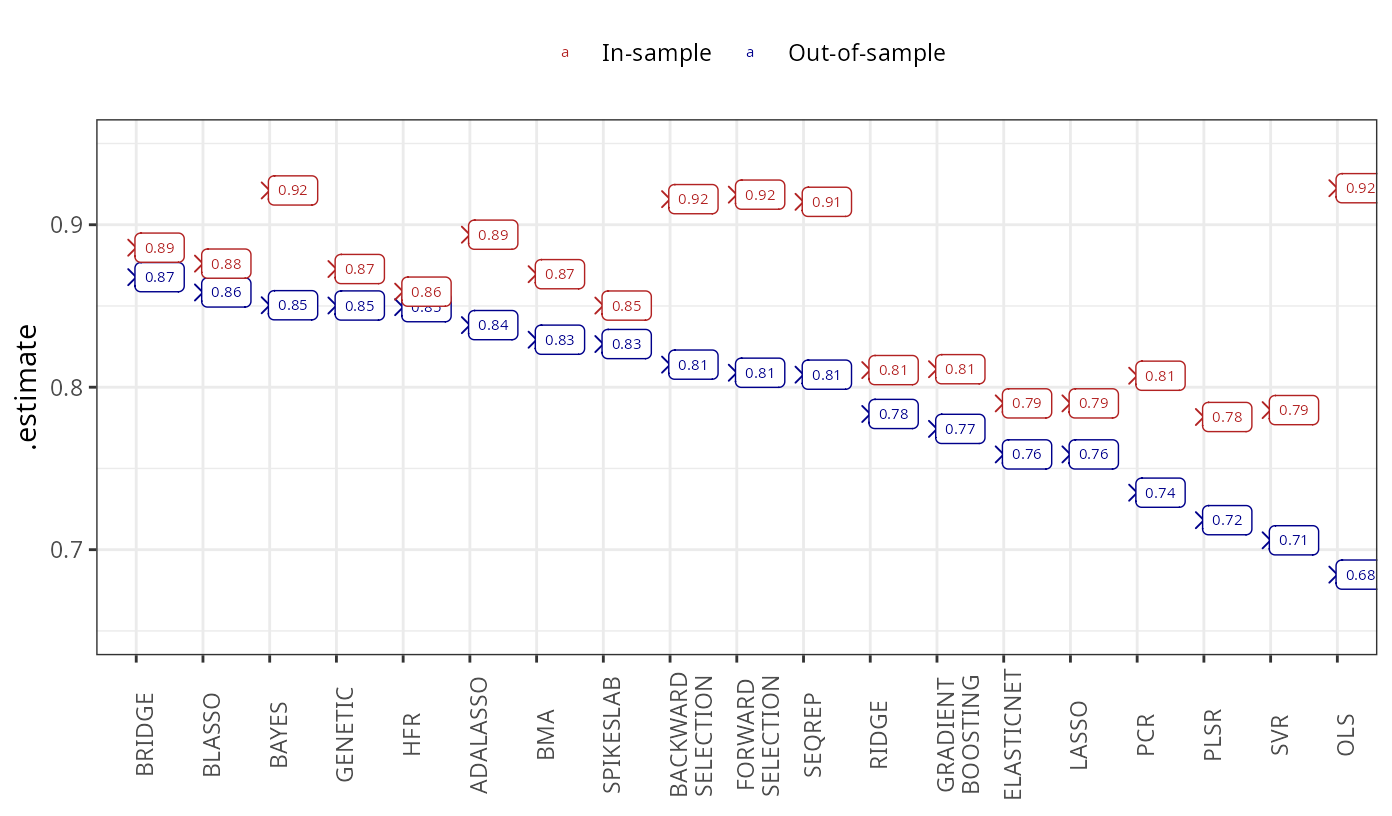
The Bayesian regression techniques overwhelmingly outperform the remaining methods, with the exception of the hierarchical feature regression, genetic algorithm and the adaptive lasso, both of which achieve relatively high out-of-sample performance. The subset selection algorithms achieve relatively good results, while the penalized and latent factor regressions perform worst. All methods improve on the OLS results.
A glimpse at the backend
tidyfit makes it exceedingly simple to fit different
regularized linear regressions. The package ensures that the input and
output of the modeling engine, tidyfit::m are standardized
and model results are comparable. For instance, whenever necessary,
features are standardized with the coefficients transformed back to the
original scale. Hyperparameter grids are set to reasonable starting
values and can be passed manually to tidyfit::m.
The package further includes a tidyfit::classify method
that assumes a binomial or multinomial response. Many of the methods
implemented can handle Gaussian and binomial responses. Furthermore, the
tidyfit::regress and tidyfit::classify methods
seamlessly integrate with grouped tibbles, making it extremely powerful
to estimate a large number of regressions for different data groupings.
Groups as well as response distributions are automatically respected by
the predict method.
Have a look at
?MASS::Bostonfor definitions of the features.↩︎Parallelizing happens at the level of cross validation slices, so always consider if the overhead of parallel computation is worth it. For instance, parallelizing will likely be very useful with
.cv = "loo_cv"but can be less useful with.cv = "vfold_cv".↩︎