library(dplyr); library(tidyr); library(purrr) # Data wrangling
library(ggplot2); library(stringr) # Plotting
library(tidyfit) # Model fitting

# Max model size
MODEL_SIZE <- 10
tidyfit packages several methods that can be used for
feature selection. These include filter,
wrapper and embedded algorithms. In
this tutorial, we will use 3 algorithms from each of these broader
categories, in order to select the top 10 best predictors of industrial
production from a macroeconomic data set of monthly US economic
indicators (FRED-MD).
The FRED-MD data set contains 134 variables characterizing the US macroeconomy with a monthly frequency and values (across all features) since the early 1990s. The data set is often used in academic research — primarily for the development of high-dimensional forecasting and nowcasting. All variables have conveniently been transformed to ensure stationarity. A description of the data as well as transformations can be found here.
The data can be downloaded using the fbi-package in
R.1 In addition to the variables included
there, I augment the ISM manufacturing PMI data (6 features), which is
no longer provided by FRED.
# Load the data
data <- readRDS("FRED-MD.rds")
Let’s shift the target to generate a forecast, and drop missing values:
data <- data |>
  arrange(date) |>
  # Shift the target by 1 month
  mutate(Target = lead(INDPRO)) |>
  drop_na() |>
  select(-date)

data
#> # A tibble: 363 × 135
#>          RPI   W875RX1 DPCERA3M086SBEA CMRMTSPLx  RETAILx    INDPRO   IPFPNSS
#>        <dbl>     <dbl>           <dbl>     <dbl>    <dbl>     <dbl>     <dbl>
#>  1  0.00165   0.000812        0.00182    0.00402 -0.00300  0.00828   0.00851
#>  2  0.00373   0.00275         0.000839   0.00664  0.00602  0.00759   0.00743
#>  3  0.00533   0.00549         0.00515   -0.00874  0.00547  0.00322   0.00550
#>  4  0.00417   0.00445         0.00270    0.0105   0.00280  0.000539 -0.00244
#>  5 -0.000796 -0.00135         0.00334    0.0133   0.00708  0.00891   0.00998
#>  6  0.00386   0.00381         0.00247   -0.0160   0.00324 -0.00557  -0.00114
#>  7 -0.00383  -0.00495         0.00649    0.0138   0.00949  0.00314  -0.000570
#>  8 -0.00492  -0.00580         0.00337    0.00404  0.00721  0.00679   0.00775
#>  9  0.00218   0.00446         0.00171    0.00170  0.00221  0.00403   0.00285
#> 10  0.0358    0.0401          0.00656    0.0154   0.0122   0.00158   0.00336
#> # ℹ 353 more rows
#> # ℹ 128 more variables: IPFINAL <dbl>, IPCONGD <dbl>, IPDCONGD <dbl>,
#> #   IPNCONGD <dbl>, IPBUSEQ <dbl>, IPMAT <dbl>, IPDMAT <dbl>, IPNMAT <dbl>,
#> #   IPMANSICS <dbl>, IPB51222S <dbl>, IPFUELS <dbl>, CUMFNS <dbl>, HWI <dbl>,
#> #   HWIURATIO <dbl>, CLF16OV <dbl>, CE16OV <dbl>, UNRATE <dbl>, UEMPMEAN <dbl>,
#> #   UEMPLT5 <dbl>, UEMP5TO14 <dbl>, UEMP15OV <dbl>, UEMP15T26 <dbl>,
#> #   UEMP27OV <dbl>, CLAIMSx <dbl>, PAYEMS <dbl>, USGOOD <dbl>, …
Feature selection algorithms
We will fit each of the feature selection algorithms using the
regress function in tidyfit, and will
iteratively build a tidyfit.models-frame below.
Filter methods
Filter methods are model-agnostic and perform univariate comparisons
between each feature and the target. They encompass the simplest (and
typically fastest) group of algorithms. One of the most basic forms of
feature selection uses Pearson’s correlation
coefficient. As with all tidyfit methods,
m("cor") fits the method. The actual correlation
coefficients will be obtained using coef():
The ReliefF algorithm is a popular
nearest-neighbors-based approach to feature selection and can be
implemented using m("relief"). The function will
automatically use the regression version (RReliefF) when executed within
a regress wrapper:
# RReliefF
algorithms_df <- algorithms_df |>
  bind_rows(
    data |>
      regress(Target ~ ., RReliefF = m("relief"))
  )
Under the hood, m("relief") is a wrapper for
CORElearn::attrEval, which bundles a large number of
selection algorithms, with estimator = "RReliefFequalK" as
the default. This default can be overridden to employ any alternative
feature selection algorithm, such as another nonparametric method called
information gain. This method first requires the
continuous target to be bucketized:
Wrapper methods
The next set of methods perform iterative feature selection. The
methods fit a model in a sequential manner, eliminating or adding
features based on some criterion of model fit or predictive accuracy. We
begin with forward selection, performed using
m("subset"). Here we can specify the target model size
directly:
# Forward Selection
algorithms_df <- algorithms_df |>
  bind_rows(
    data |>
      regress(Target ~ .,
              `Forward Selection` = m("subset", method = "forward", nvmax = MODEL_SIZE))
  )
The opposite of forward selection is backward elimination. This method is also implemented using the “subset” wrapper:
# Backward Elimination
algorithms_df <- algorithms_df |>
  bind_rows(
    data |>
      regress(Target ~ .,
              `Backward Elimination` = m("subset", method = "backward", nvmax = MODEL_SIZE))
  )
The final sequential algorithm examined here is minimum
redundancy, maximum relevance (MRMR). The algorithm selects
features based on the dual objective of maximizing the relevance for the
target, while minimizing redundant information in the feature set.
m("mrmr") is a wrapper for
mRMRe::mRMR.ensemble:
Embedded methods
The last group of feature selection algorithms, embedded methods, combine model selection and estimation into a single step — for instance, by forcing a subset of the parameter weights to be zero. The LASSO does this by introducing an -penalty on the parameters. Here we will use an expanding window grid search validation to determine the optimal penalty2:
# LASSO
algorithms_df <- algorithms_df |>
  bind_rows(
    data |>
      regress(Target ~ .,
              `LASSO` = m("lasso", pmax = MODEL_SIZE + 1),
              .cv = "rolling_origin",
              .cv_args = list(initial = 120, assess = 24, skip = 23)
              )
  )
Bayesian model averaging takes a different approach,
sampling a large number of models and using Bayes’ rule to compute a
posterior inclusion probability for each feature. m("bma")
is a wrapper for BMS::bms:
# BMA
algorithms_df <- algorithms_df |>
  bind_rows(
    data |>
      regress(Target ~ .,
              BMA = m("bma", burn = 10000, iter = 100000,
                      mprior.size = MODEL_SIZE, mcmc = "rev.jump"))
  )
Last, but not least, Random Forests importance is a
popular machine learning technique for model selection. We estimate a
simple random forest using default settings, with m("rf"),
which is a wrapper for the randomForest-package. Note that
importance = TRUE by default, thus feature importances are
computed and can be accessed using coef:
Extracting the top models
All information needed to select the top 10 features for each
algorithm can be obtained using coef(algorithms_df) and
unnesting the additional information stored in
model_info:
Some algorithms return more than the maximum 10 variables. For instance, the filter methods (correlation, RReliefF and information gain) return a score for each feature. The below code chunk selects the top 10 features for each algorithm:
model_df <- coef_df |>
  # Always remove the intercept
  filter(term != "(Intercept)") |>

  mutate(selected = case_when(
    # Extract top 10 largest scores
    model %in% c("Correlation", "RReliefF", "Information Gain") ~
      rank(-abs(estimate)) <= MODEL_SIZE,
    # BMA features are selected using the posterior inclusion probability
    model == "BMA" ~ rank(-pip) <= MODEL_SIZE,
    # The RF importance is stored in a separate column (%IncMSE)
    model == "RF Importance" ~ rank(-importance) <= MODEL_SIZE,
    # For all other methods keep all features
    TRUE ~ TRUE
  )) |>

  # Keep only included terms
  filter(selected) |>
  select(model, term)
Before examining the results, we will also add a domain expert. Here I simply add those features that are included in the US Conference Board Composite Leading Indicator and are available in our data set:
model_df <- model_df |>
  bind_rows(tibble(
    model = "Domain Expert",
    term = c("NAPMNOI", "ANDENOx", "CLAIMSx", "ACOGNO",
             "S&P 500", "T10YFFM", "PERMIT", "AWHMAN")
  ))
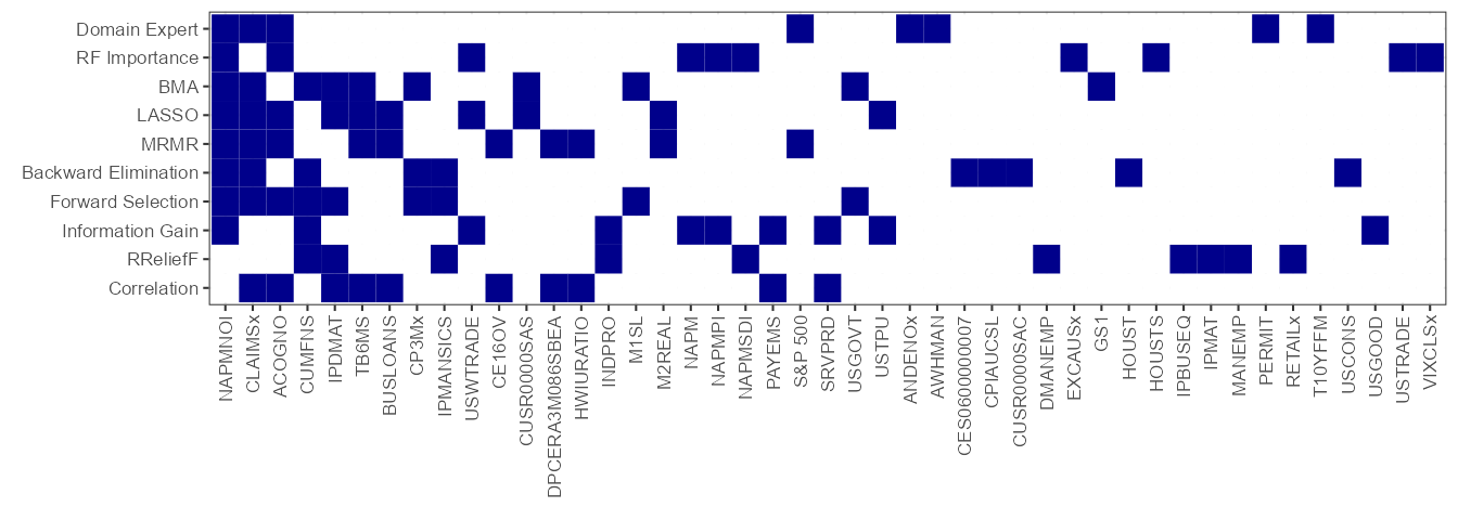
Now, let’s examine the models selected by each of the various algorithms:
model_df |>
  # Add 'FALSE' entries, when a feature is not selected
  mutate(selected = TRUE) |>
  spread(term, selected) |>
  gather("term", "selected", -model) |>
  # Plotting color
  mutate(selected = ifelse(is.na(selected), "white", "darkblue")) |>
  # Fix plotting order
  group_by(term) |>
  mutate(selected_sum = sum(selected=="darkblue")) |>
  ungroup() |>
  arrange(desc(selected_sum)) |>
  mutate(term = factor(term, levels = unique(term))) |>
  mutate(model = factor(model, levels = unique(model_df$model))) |>
  ggplot(aes(term, model)) +
  geom_tile(aes(fill = selected)) +
  theme_bw(8) +
  scale_fill_identity() +
  xlab(element_blank()) + ylab(element_blank()) +
  theme(axis.text.x = element_text(angle = 90, vjust = 0.5, hjust=1))
There is quite a lot of disagreement between different feature
selection algorithms. We can develop an understanding of the type of
information selected by each algorithm by examining how well each
feature set explains the target using the
-statistic.
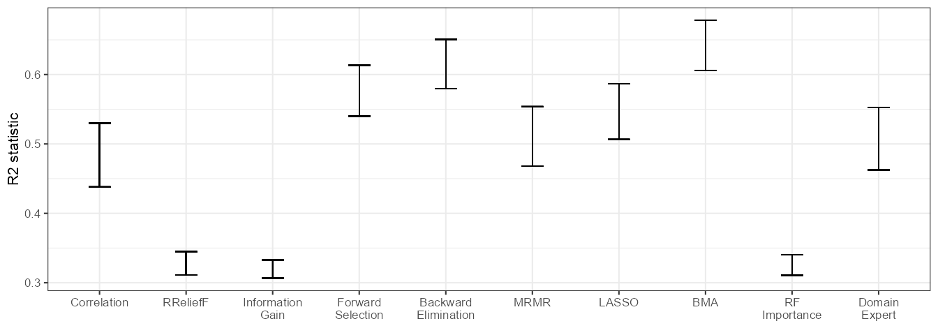
To get a sense of the sample stability, we generate bootstrap samples
and regress the target onto each model. Note that it is important to set
.force_cv = TRUE below, since m("lm") does not
have hyperparameters and thus ignores the .cv argument by
default.
model_names <- unique(model_df$model)

# Retrieve selected variables
selected_vars_list <- model_names |>
  map(function(mod) {
    model_df |>
      filter(model == mod) |>
      pull(term)
  })
names(selected_vars_list) <- model_names

# Bootstrap resampling & regression
boot_models_df <- selected_vars_list |>
  map_dfr(function(selected_vars) {
    data |>
      select(all_of(c("Target", selected_vars))) |>

      regress(Target ~ .,
              # Use linear regression
              m("lm"),
              # Bootstrap settings (see ?rsample::bootstraps)
              .cv = "bootstraps", .cv_args = list(times = 100),
              # Make sure the results for each slice are returned
              .force_cv = T, .return_slices = T)
  }, .id = "model")

# Finally, extract R2 from the model results
boot_df <- boot_models_df |>
  mutate(R2 = map_dbl(model_object, function(obj) summary(obj)$r.squared)) |>
  select(model, R2)
boot_df |>
  group_by(model) |>
  mutate(upper = mean(R2) + 2 * sd(R2) / sqrt(n()),
         lower = mean(R2) - 2 * sd(R2) / sqrt(n())) |>
  mutate(model = str_wrap(model, 10)) |>
  mutate(model = factor(model, levels = str_wrap(unique(model_df$model), 10))) |>
  ggplot(aes(model)) +
  geom_errorbar(aes(ymin = lower, ymax = upper), linewidth = 0.25, width = 0.25) +
  theme_bw(8) +
  xlab(element_blank()) + ylab("R2 statistic")
The filter methods as well as RF Importance tend to explain a relatively small proportion of the response variation, while BMA and subset selection algorithms perform best.
See
?fbi::fredmd.↩︎See
?rsample::rolling_originfor details↩︎