Multinomial Classification

library(dplyr); library(tidyr); library(purrr) # Data wrangling
library(ggplot2); library(stringr) # Plotting
library(tidyfit)   # Auto-ML modeling

Multinomial classification is possible in tidyfit using the methods powered by glmnet, e1071 and randomForest (LASSO, Ridge, ElasticNet, AdaLASSO, SVM and Random Forest). Currently, none of the other methods support multinomial classification.¹ When the response variable contains more than 2 classes, classify automatically uses a multinomial response for the above-mentioned methods.

Here’s an example using the built-in iris dataset:

data("iris")

# For reproducibility
set.seed(42)
ix_tst <- sample(1:nrow(iris), round(nrow(iris)*0.2))

data_trn <- iris[-ix_tst,]
data_tst <- iris[ix_tst,]

as_tibble(iris)
#> # A tibble: 150 × 5
#>    Sepal.Length Sepal.Width Petal.Length Petal.Width Species
#>           <dbl>       <dbl>        <dbl>       <dbl> <fct>  
#>  1          5.1         3.5          1.4         0.2 setosa 
#>  2          4.9         3            1.4         0.2 setosa 
#>  3          4.7         3.2          1.3         0.2 setosa 
#>  4          4.6         3.1          1.5         0.2 setosa 
#>  5          5           3.6          1.4         0.2 setosa 
#>  6          5.4         3.9          1.7         0.4 setosa 
#>  7          4.6         3.4          1.4         0.3 setosa 
#>  8          5           3.4          1.5         0.2 setosa 
#>  9          4.4         2.9          1.4         0.2 setosa 
#> 10          4.9         3.1          1.5         0.1 setosa 
#> # ℹ 140 more rows

Penalized classification algorithms to predict `Species`

The code chunk below fits the above mentioned algorithms on the training split, using a 10-fold cross validation to select optimal penalties. We then obtain out-of-sample predictions using predict. Unlike binomial classification, the fit and pred objects contain a class column with separate coefficients and predictions for each class. The predictions sum to one across classes:

fit <- data_trn |>
  classify(Species ~ ., 
           LASSO = m("lasso"), 
           Ridge = m("ridge"), 
           ElasticNet = m("enet"), 
           AdaLASSO = m("adalasso"),
           SVM = m("svm"),
           `Random Forest` = m("rf"),
           `Least Squares` = m("ridge", lambda = 1e-5), 
           .cv = "vfold_cv")

pred <- fit |>
  predict(data_tst)

Note that we can add unregularized least squares estimates by setting lambda = 0 (or very close to zero).

Next, we can use yardstick to calculate the log loss accuracy metric and compare the performance of the different models:

metrics <- pred |>
  group_by(model, class) |>
  mutate(row_n = row_number()) |>
  spread(class, prediction) |>
  group_by(model) |>
  yardstick::mn_log_loss(truth, setosa:virginica)

metrics |>
  mutate(model = str_wrap(model, 11)) |>
  ggplot(aes(model, .estimate)) +
  geom_col(fill = "darkblue") +
  theme_bw() +
  theme(axis.title.x = element_blank())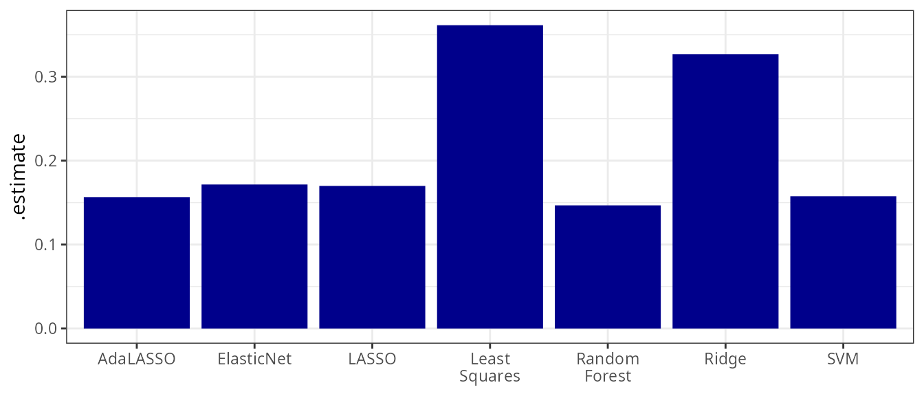

The least squares estimate performs poorest, while the random forest (nonlinear) and the support vector machine (SVM) achieve the best results. The SVM is estimated with a linear kernel by default (use kernel = <chosen_kernel> to use a different kernel).

Feature selection methods such as relief or chisq can be used with multinomial response variables. I may also add support for multinomial classification with mboost in future.↩︎

Penalized classification algorithms to predict Species

Penalized classification algorithms to predict `Species`